12 Clustering Using K-means
Natural Groups are best described, not by any Definition which marks their boundaries, but by a Type which marks their center.
Suppose a retailer has detailed records of customer purchases but no predefined customer segments. The data describe how customers differ across many products, yet there are no predefined labels indicating how they should be grouped. Similar situations arise in healthcare, digital services, and scientific research, where many characteristics may be observed without predefined categories. In such settings, the task is not to predict a known outcome, but to examine whether patterns of similarity among the observations provide a useful way to organize the data.
Clustering is designed for exactly this situation. It groups observations according to similarity, so that observations within the same cluster resemble one another more closely than observations in different clusters. In this way, clustering can summarize a complex dataset through a smaller number of groups that may be easier to interpret and investigate. Among the many methods available for this purpose, K-means is one of the most widely used and provides the main focus of this chapter.
Unlike the supervised learning methods developed in the preceding modeling chapters, which use a known response variable for classification or regression, clustering seeks structure directly from the observed features. This shift from prediction to structure discovery distinguishes clustering from the supervised methods considered earlier in the book.
Clustering belongs to the broader family of unsupervised learning methods introduced in Section 1.10. It does not recover fixed or guaranteed “true” groups hidden in the data. Instead, it provides an analytical summary of multivariate structure that can support interpretation, hypothesis generation, and subsequent analysis. Its role in the Data Science Workflow presented in Chapter 1 (Figure 1.1) therefore depends on the analytical objective. During Data Understanding and Exploration, clustering may be used to reveal possible patterns or subgroups that warrant further investigation. When segmentation itself is the objective of the analysis, however, clustering serves as the primary method in the Modeling stage. In both roles, the resulting groups should be interpreted cautiously and in light of the problem being studied.
What This Chapter Covers
This chapter develops clustering as an unsupervised learning approach for identifying and interpreting structure in data without a response variable. Because there is no known outcome against which predictions can be compared, assessing clustering solutions places greater emphasis on internal measures, stability, and substantive interpretability.
We begin by introducing the goals of cluster analysis and clarifying how clustering differs from classification. We then examine how similarity is defined, with particular attention to distance measures for numerical data. Next, we develop the K-means algorithm in more depth, including its objective function, iterative updating mechanism, and practical issues such as local minima, instability across runs, cluster quality, and situations in which K-means may perform poorly.
Before turning to the case study, we briefly introduce several alternatives to K-means, including hierarchical clustering, density-based clustering, and mixture models. We then apply the main ideas of the chapter in a case study using the wholesale_customers dataset from the liver package, where K-means is used to segment customers according to purchasing behavior. Exercises at the end of the chapter reinforce both conceptual understanding and practical implementation.
By the end of the chapter, you should be able to explain the purpose of clustering, apply K-means to data without a known response variable, make informed choices about data preparation and the number of clusters, assess clustering solutions critically, and interpret the resulting groups in a domain-aware and appropriately cautious way.
12.1 What is Cluster Analysis?
Cluster analysis is an unsupervised learning approach that groups observations into clusters based on their similarity. The general aim is to form groups in which observations within the same cluster are more similar to one another than to observations in different clusters. In contrast to supervised learning, clustering does not rely on labeled examples or a known response variable. Instead, it is used to explore whether the data exhibit meaningful internal structure.
To clarify this setting, it is helpful to contrast clustering with classification, introduced in Chapters 4 and 6. Classification assigns observations to predefined categories using labeled training data. Clustering, by contrast, constructs groups directly from the observed features. These groupings are not known in advance, and they should not automatically be interpreted as true categories hidden in the data. Unless there is strong external evidence supporting such an interpretation, clusters are better viewed as analytical summaries of multivariate patterns rather than as discovered facts.
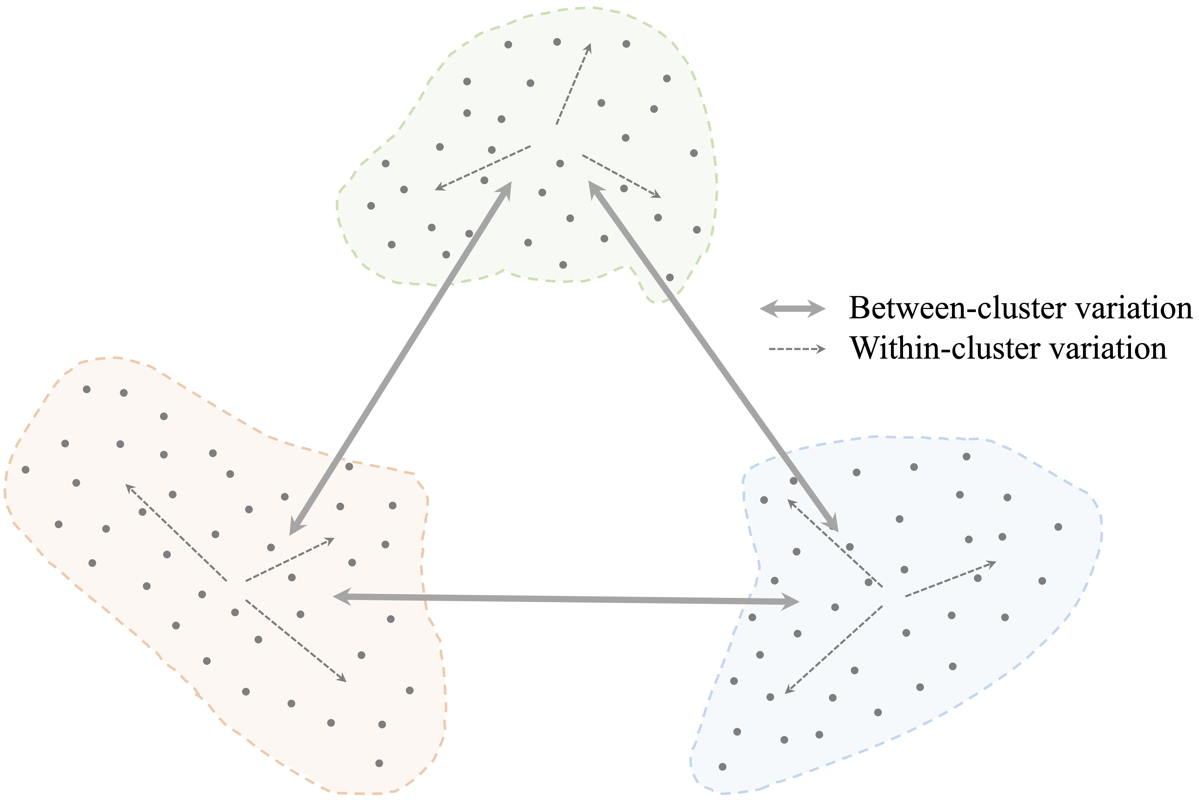
The objective of clustering is often described in terms of high intra-cluster similarity and low inter-cluster similarity. In other words, a useful clustering places similar observations together while separating dissimilar ones into different groups. This principle is illustrated in Figure 12.1, where compact and well-separated groups correspond to a stronger clustering solution.
Although clustering is often introduced as an exploratory technique, its role extends beyond description alone. Cluster assignments can help summarize large datasets, support interpretation, guide hypothesis generation, and provide derived features for downstream analyses. At the same time, clustering results should always be interpreted cautiously. Different algorithms, similarity measures, preprocessing choices, and numbers of clusters can lead to different solutions, and no single clustering should automatically be regarded as definitive. In practice, the value of clustering lies not in revealing fixed categories, but in offering a useful and interpretable simplification of complex multivariate data.
These considerations lead naturally to a central question: how do clustering algorithms decide whether two observations are similar? We address this next.
Measuring Similarity in Clustering
At the core of clustering lies a fundamental question: how similar are two observations? Clustering algorithms address this question through similarity measures or distance measures, which quantify how closely observations resemble one another. The choice of similarity measure is not merely a technical detail. It is a modeling decision that directly shapes the cluster structure an algorithm can detect.
For numerical data, the most commonly used measure is Euclidean distance, which represents the straight-line distance between two observations in feature space. This measure was introduced earlier in the context of the k-Nearest Neighbors algorithm (Section 4.4). In clustering, Euclidean distance plays a similar role by determining which observations are close enough to be grouped together. Formally, the Euclidean distance between two observations \(x = (x_1, x_2, \ldots, x_n)\) and \(y = (y_1, y_2, \ldots, y_n)\) with \(n\) features is defined as \[ \text{dist}(x, y) = \sqrt{\sum_{i=1}^n (x_i - y_i)^2}. \]
Euclidean distance works naturally when the variables are numerical, continuous, and placed on comparable scales. In such settings, geometric closeness provides a reasonable notion of similarity. However, Euclidean distance is sensitive to scale: variables with larger numerical ranges can dominate the calculation and, in turn, strongly influence the resulting clusters. This is why distance-based clustering methods often require careful preprocessing before the analysis begins.
In practice, similarity depends not only on the distance formula itself, but also on how the data are represented. Features measured on different scales may need to be standardized or rescaled. Skewed variables may benefit from transformation. Categorical variables require an appropriate representation or a distance measure designed for categorical or mixed-type data. These decisions form part of the Data Preparation for Modeling stage introduced in Chapter 3. In clustering, they are especially important because they directly affect the geometry of the data and therefore the groups that emerge. We return to these issues in the case study later in this chapter.
Although Euclidean distance is widely used, it is not always appropriate. For example, it is less suitable for sparse data, directional data, text data, or data containing a mixture of numerical and categorical variables. In such cases, alternative measures may better reflect the notion of similarity relevant to the problem. Manhattan distance may be useful when absolute coordinate differences are of primary interest, whereas cosine similarity is often more appropriate when the direction of a feature vector matters more than its magnitude.
These considerations are especially important for K-means clustering. K-means relies on numerical features, Euclidean geometry, and cluster means, so its behavior is tightly linked to how the variables are prepared. For K-means, preprocessing is therefore not incidental: it largely determines what kind of cluster structure the algorithm can detect.
12.2 K-means Clustering
How does an algorithm decide which observations belong together? K-means clustering addresses this question by representing each cluster through a centroid and assigning observations to the nearest centroid based on distance. By alternating between assignment and update steps, the algorithm gradually refines both the cluster memberships and their representative centers, partitioning the observations into \(k\) clusters.
More formally, K-means seeks a partition that minimizes the within-cluster sum of squares: \[ \sum_{r=1}^{k}\sum_{i \in C_r} \lVert x_i - \mu_r \rVert^2, \] where \(C_r\) denotes the set of observations assigned to cluster \(r\), and \(\mu_r\) is the centroid of that cluster. In other words, the algorithm aims to form clusters in which observations lie as close as possible to their assigned centroids. Because each centroid is defined as a mean, K-means is naturally suited to numerical data. The assignment and update steps of the algorithm can therefore be understood as an iterative procedure for reducing this objective function.
The K-means algorithm requires the number of clusters, \(k\), to be specified in advance. Given a choice of \(k\), the algorithm proceeds as follows:
Initialization: Select \(k\) initial cluster centers, typically at random.
Assignment: Assign each observation to the nearest cluster center.
Update: Recompute each cluster center as the mean of the observations assigned to it.
Iteration: Repeat the assignment and update steps until the assignments stabilize and the objective function no longer decreases.
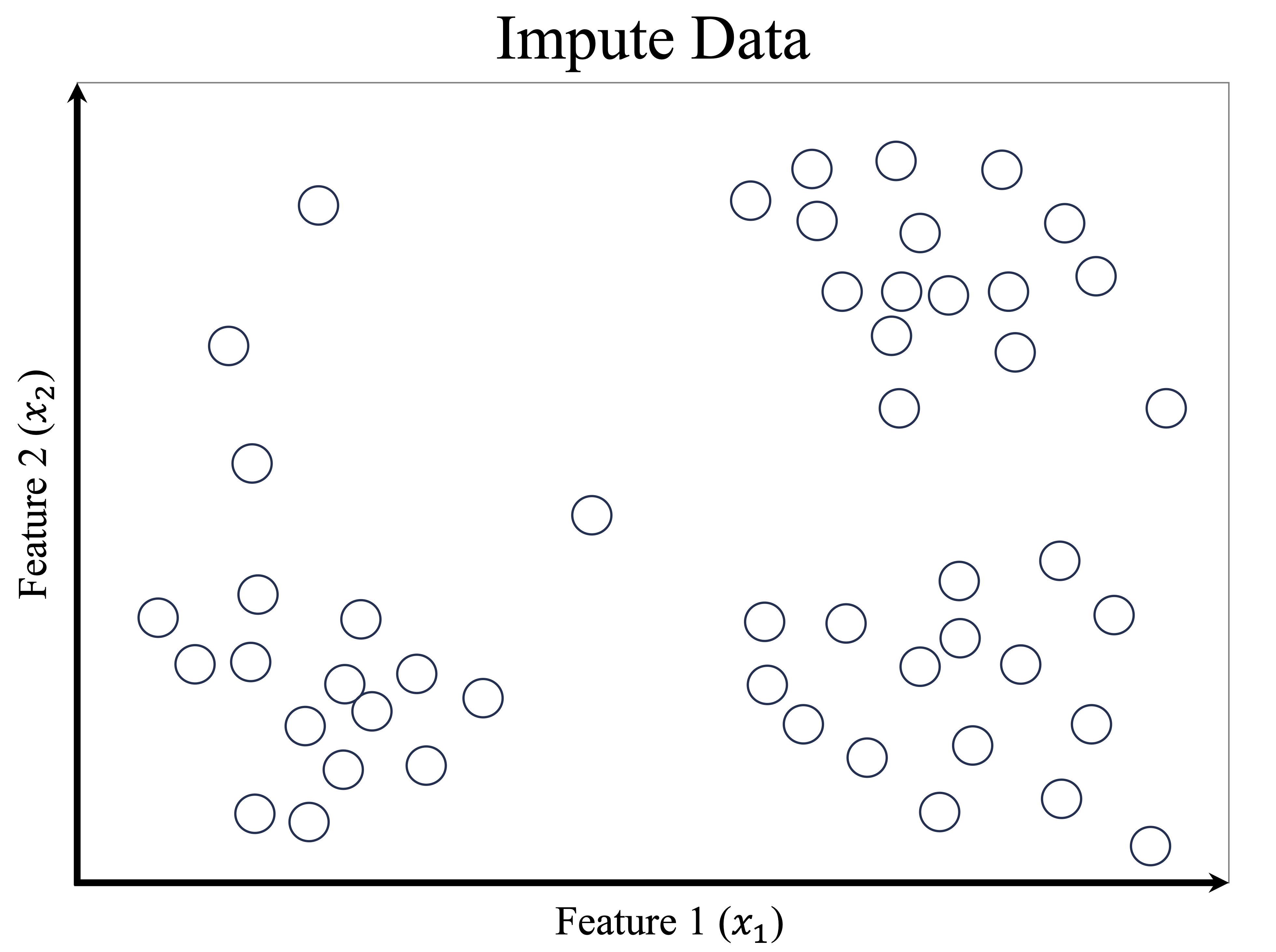
To illustrate these steps, consider a dataset consisting of 50 observations with two features, \(x_1\) and \(x_2\), shown in Figure 12.2. The goal is to partition the data into three clusters.
The sequence of panels in Figure 12.3 illustrates how K-means proceeds. The algorithm begins by selecting three initial cluster centers, shown as red stars. Each observation is then assigned to its nearest center, which partitions the feature space into regions defined by proximity to the current centroids. After this assignment step, the cluster centers are updated by computing the mean of the observations currently assigned to each cluster. These updated centroids induce a new partition of the data, and some observations may therefore be reassigned. As this process continues, the value of the within-cluster sum of squares decreases, the centroid locations become more stable, and the clustering gradually settles into a final solution.
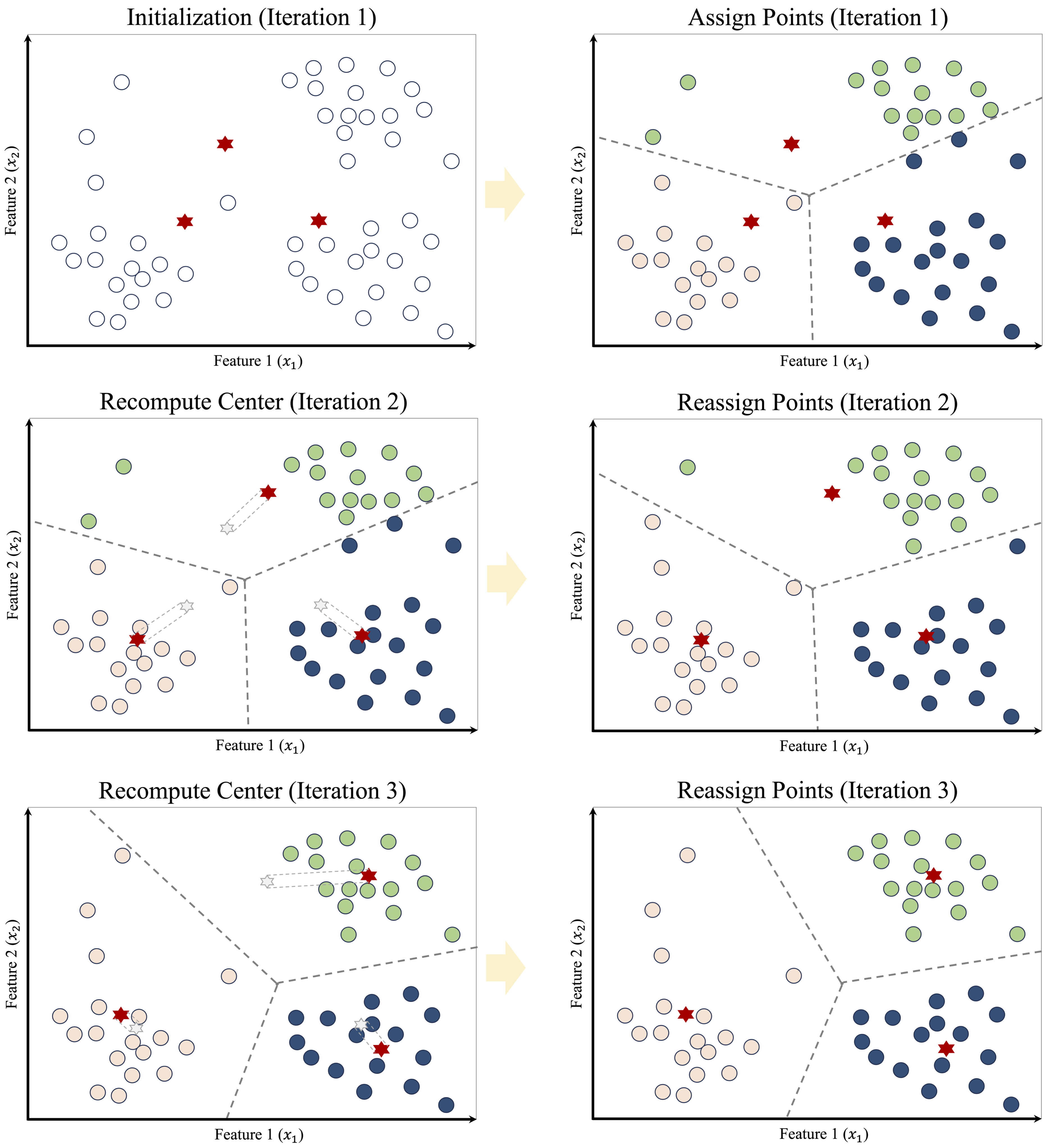
Once the algorithm has converged, the results can be summarized in two complementary ways: the cluster assignments, which indicate the group membership of each observation, and the cluster centroids, which serve as representative profiles of the clusters. These centroids are especially useful in applications such as customer segmentation, image compression, and document clustering, where the goal is to simplify the data while preserving meaningful structure. However, convergence alone should not be taken as evidence that the clustering is uniquely correct or substantively meaningful. It simply means that, for the chosen initialization, the assignment and update steps have reached a stable configuration.
Despite its simplicity and efficiency, K-means has important limitations. Because the algorithm starts from an initial set of centroids and iteratively improves the solution, it generally converges to a local minimum of the objective function rather than guaranteeing the global minimum. As a result, different random initializations can produce different final clusterings, which makes repeated runs and stability checks important in practice. K-means works best when clusters are reasonably compact, roughly spherical, and similarly scaled. It is also sensitive to outliers and skewed distributions, both of which can distort centroid locations and lead to less representative cluster assignments. More broadly, the method may perform poorly when clusters are elongated, highly overlapping, very unequal in size, or not well represented by their means. These limitations reflect the fact that K-means searches for clusters using Euclidean distance and cluster centroids, so it is most effective when that geometric representation aligns well with the structure of the data. For this reason, fitting a K-means model is only the beginning of the analysis: we must still consider whether the resulting partition is stable, coherent, and substantively interpretable. We return to these questions in the next section, where we discuss how to choose the number of clusters and how to assess the quality of a clustering solution.
12.3 Choosing the Number of Clusters
A central challenge in applying K-means clustering is choosing the number of clusters, \(k\). This choice has a direct impact on the resulting partition: too few clusters may obscure meaningful structure, whereas too many may fragment the data and reduce interpretability. Unlike supervised learning, clustering does not provide an external ground truth against which different values of \(k\) can be evaluated directly. As a result, the choice of \(k\) is not purely objective, but neither is it arbitrary. In practice, it is informed by a combination of quantitative criteria, stability considerations, and substantive interpretability.
A useful way to think about this decision is as a hierarchy of evidence. First, internal criteria such as within-cluster variation, silhouette scores, or the gap statistic can help identify values of \(k\) that appear reasonable from the data alone. Second, it is often helpful to examine how stable the clustering remains across nearby choices of \(k\) or across repeated runs of the algorithm. Third, and most importantly, the final choice should be interpretable in the context of the application. A clustering that looks appealing numerically but yields segments with little practical meaning may not be useful in practice.
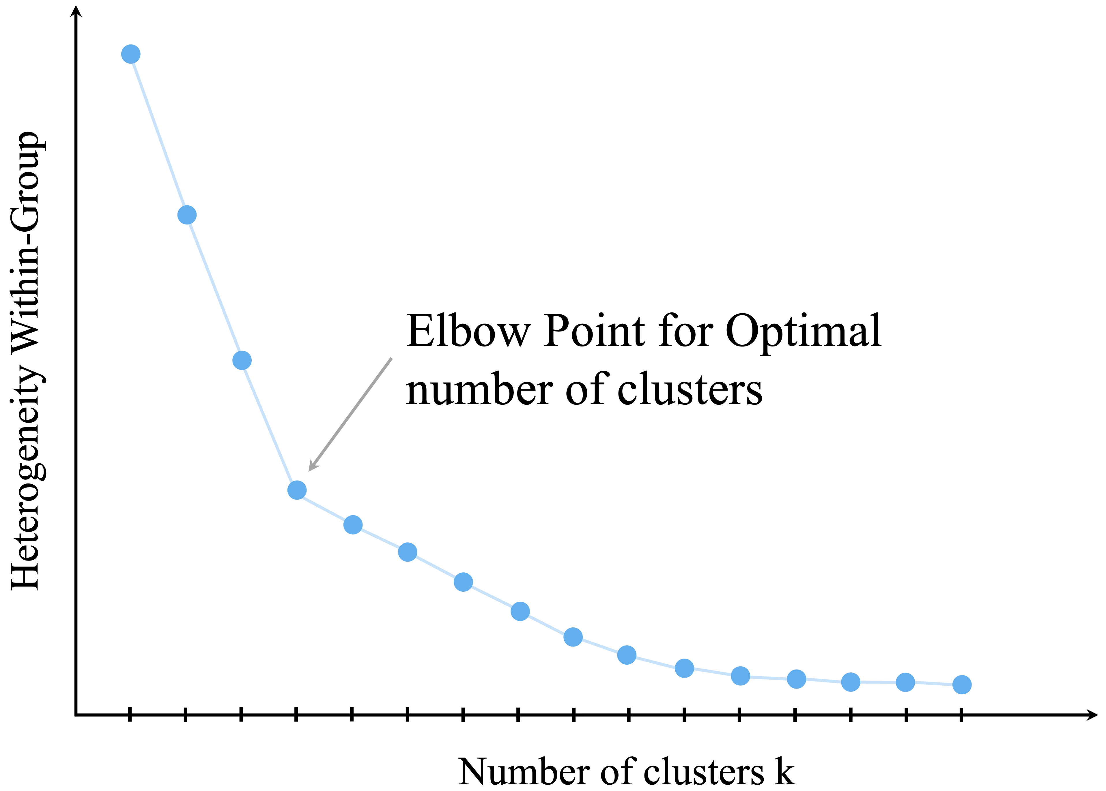
One widely used internal criterion is the elbow method, which examines how within-cluster variation changes as the number of clusters increases. As additional clusters are introduced, the total within-cluster sum of squares (WCSS) decreases because the observations are partitioned into smaller and more homogeneous groups. However, the marginal improvement typically becomes smaller as \(k\) increases. The aim is to identify a point of diminishing returns, often referred to as the elbow, beyond which adding more clusters yields only modest reductions in within-cluster variation.
This idea is illustrated in Figure 12.4, which plots WCSS against the number of clusters. A visible bend in the curve suggests a value of \(k\) that balances model simplicity with within-cluster cohesion.
Although the elbow method is intuitive and widely used, it should be treated as a heuristic rather than as a definitive rule. Some datasets exhibit no clear elbow, and different analysts may reasonably identify different bend points in the same curve. For this reason, it is often useful to supplement the elbow plot with other internal criteria. The silhouette score, for example, evaluates how well observations fit within their assigned clusters relative to other clusters, while the gap statistic compares the observed clustering structure to that expected under a suitable reference distribution.
Even when such criteria are helpful, they do not remove the need for judgment. In practice, it is often informative to compare clustering solutions across a small range of values, such as \(k = 2\), \(3\), and \(4\), and to examine whether the resulting groups remain reasonably stable and interpretable. If small changes in \(k\) produce radically different results, this may indicate that the data do not support a clear segmentation. If several nearby choices lead to similar patterns, confidence in the general structure may be strengthened.
Ultimately, the goal is not to discover a single “correct” value of \(k\), but to choose a solution that is coherent, stable, and useful for the analytical objective at hand. At the same time, the question of how many clusters to use arises within a particular clustering framework. Before turning to the case study, we therefore briefly step back and consider several alternatives to K-means that rest on different assumptions about what a cluster is.
12.4 Beyond K-means
K-means is one of the most widely used clustering methods because it is conceptually simple, computationally efficient, and easy to interpret. At the same time, it is not appropriate for every clustering problem. As we have seen, K-means works best when the data are numerical, the clusters are reasonably compact, and the group structure can be represented well by cluster centroids. When these conditions are not met, other clustering approaches may provide a more useful description of the data.
In this section, we briefly introduce three important alternatives to K-means: hierarchical clustering, density-based clustering, and mixture models. The goal is not to develop these methods in detail, but to highlight how different clustering algorithms embody different assumptions about what a cluster is.
Hierarchical Clustering
Hierarchical clustering takes a different approach from K-means. Rather than requiring the number of clusters to be fixed in advance, it builds a nested sequence of groupings. In its agglomerative form, which is the version most commonly introduced in practice, the algorithm begins by treating each observation as its own cluster and then repeatedly merges the two closest clusters until all observations belong to a single group.
The result is often displayed as a dendrogram, which is a tree-like diagram showing how clusters are merged across steps. By cutting the dendrogram at a chosen height, we can obtain different numbers of clusters. This makes hierarchical clustering especially useful when we want to explore the data at several levels of granularity rather than commit immediately to a single value of \(k\).
A key difference from K-means is that hierarchical clustering does not rely on cluster centroids. Instead, it depends on a notion of distance between clusters, called a linkage criterion, such as single linkage, complete linkage, or average linkage. Different linkage choices can lead to quite different clustering structures. Hierarchical clustering is often attractive for exploratory work, but it can be sensitive to noise and may become computationally demanding for very large datasets.
Density-Based Clustering
Density-based clustering defines clusters as regions of high data density separated by regions of lower density. This is a very different view from K-means, which searches for compact groups around centroids. A major advantage of density-based methods is that they can detect clusters with irregular or non-spherical shapes.
Methods such as DBSCAN are particularly useful when the data contain noise or outliers. Rather than forcing every observation into a cluster, density-based clustering can label some observations as noise if they do not belong to any sufficiently dense region. This is often desirable in applications where unusual cases should remain separate rather than distort the clustering.
Density-based methods are therefore appealing when the data contain curved, elongated, or unevenly shaped groups that K-means would represent poorly. Their performance, however, depends on tuning parameters that define what counts as a dense region, and these choices can be challenging when the data have varying densities across clusters.
Mixture Models
Mixture models provide a probabilistic perspective on clustering. Instead of assigning each observation deterministically to a single cluster, they assume that the data arise from a mixture of underlying probability distributions. In this framework, each cluster corresponds to one component of the mixture, and each observation has a probability of belonging to each component.
This approach is more flexible than K-means because it allows us to model uncertainty in cluster membership. It is especially useful when cluster boundaries are not sharp or when we want a softer notion of grouping. Gaussian mixture models are a common example for numerical data. They can represent clusters with different shapes, sizes, and orientations more naturally than K-means, which relies on Euclidean distance and cluster means.
At the same time, mixture models require stronger modeling assumptions, since we must specify a probability model for the data. They are also typically more computationally demanding than K-means and may be more difficult to fit and interpret in introductory settings.
Taken together, these methods illustrate an important general point: there is no single clustering algorithm that is best for all datasets. Different methods reflect different assumptions about cluster shape, noise, uncertainty, and scale. In this chapter, we focus on K-means because it provides a useful and accessible foundation for thinking about clustering. We now return to that method in a case study, where we illustrate how K-means can be applied in practice when the data are numerical and the resulting segments can be interpreted meaningfully.
For readers interested in a broader treatment of clustering methods in R, including hierarchical, non-hierarchical, and model-based approaches, see Giordani, Ferraro, and Martella (Giordani et al. 2020).
12.5 Case Study: Segmenting Wholesale Customers by Purchasing Behavior
Why do some wholesale customers spend heavily on fresh products, while others concentrate more on grocery items, milk, or detergents and paper goods? In this case study, we use K-means clustering to examine whether such purchasing patterns give rise to meaningful customer segments.
Using the wholesale_customers dataset from the liver package, we investigate whether groups of customers with similar purchasing profiles emerge from the data. We begin by examining the customer data and identifying the variables that will define purchasing similarity. We then prepare the spending variables for clustering, consider a suitable number of clusters, fit a K-means model, and assess and interpret the resulting customer segments.
Analytical Objective and Dataset
The aim of this analysis is to identify customer segments based on similarities in purchasing behavior. The wholesale_customers dataset contains 440 customers and 8 variables. Six variables record annual spending in major product categories: fresh, milk, grocery, frozen, detergents_paper, and delicassen. These spending variables provide the purchasing profiles on which the clustering will be based.
The remaining two variables, channel and region, describe the type of customer and the geographical area. They are not used as inputs to the K-means algorithm. Instead, they are retained as external descriptive variables that can help interpret the clusters after they have been formed. This is a substantive analytical choice: the clusters are constructed from purchasing behavior alone, while channel and region provide additional context for understanding the resulting customer segments.
We begin by loading the dataset and examining its structure and summary statistics:
library(liver)
data(wholesale_customers)

str(wholesale_customers)
   'data.frame':    440 obs. of  8 variables:
    $ fresh           : int  12669 7057 6353 13265 22615 9413 12126 7579 5963 6006 ...
    $ milk            : int  9656 9810 8808 1196 5410 8259 3199 4956 3648 11093 ...
    $ grocery         : int  7561 9568 7684 4221 7198 5126 6975 9426 6192 18881 ...
    $ frozen          : int  214 1762 2405 6404 3915 666 480 1669 425 1159 ...
    $ detergents_paper: int  2674 3293 3516 507 1777 1795 3140 3321 1716 7425 ...
    $ delicassen      : int  1338 1776 7844 1788 5185 1451 545 2566 750 2098 ...
    $ channel         : Factor w/ 2 levels "Horeca","Retail": 2 2 2 1 2 2 2 2 1 2 ...
    $ region          : Factor w/ 3 levels "Lisbon","Oporto",..: 3 3 3 3 3 3 3 3 3 3 ...
summary(wholesale_customers)
        fresh             milk          grocery          frozen        detergents_paper    delicassen        channel
    Min.   :     3   Min.   :   55   Min.   :    3   Min.   :   25.0   Min.   :    3.0   Min.   :    3.0   Horeca:298
    1st Qu.:  3128   1st Qu.: 1533   1st Qu.: 2153   1st Qu.:  742.2   1st Qu.:  256.8   1st Qu.:  408.2   Retail:142
    Median :  8504   Median : 3627   Median : 4756   Median : 1526.0   Median :  816.5   Median :  965.5
    Mean   : 12000   Mean   : 5796   Mean   : 7951   Mean   : 3071.9   Mean   : 2881.5   Mean   : 1524.9
    3rd Qu.: 16934   3rd Qu.: 7190   3rd Qu.:10656   3rd Qu.: 3554.2   3rd Qu.: 3922.0   3rd Qu.: 1820.2
    Max.   :112151   Max.   :73498   Max.   :92780   Max.   :60869.0   Max.   :40827.0   Max.   :47943.0
       region
    Lisbon: 77
    Oporto: 47
    Other :316
The dataset contains no missing values, so no imputation is required. The six spending variables are numerical and nonnegative, making them suitable candidates for a distance-based analysis. Their summary statistics also reveal substantial differences in scale and large gaps between typical and maximum spending values, indicating strong right-skewness and some unusually large observations.
These characteristics are important for K-means because the method relies on Euclidean distance and cluster means. Variables with larger numerical ranges can exert disproportionate influence on the distance calculations, while highly skewed distributions and very large observations can strongly affect the cluster centroids. The spending variables therefore require careful preparation before they are used to define customer similarity.
Data Preparation for Clustering
We first extract the six spending variables that will define the customer purchasing profiles:
selected_variables = c("fresh", "milk", "grocery", "frozen", "detergents_paper", "delicassen")
customers_subset = wholesale_customers[, selected_variables]
As observed above, the spending variables are strongly right-skewed: many customers have relatively modest expenditures, whereas a smaller number spend substantially more. If the raw values are used directly, these large observations can have considerable influence on Euclidean distances and the resulting cluster centroids.
To reduce this skewness, we apply a logarithmic transformation using log1p(), which computes \(\log(1+x)\). This transformation is well suited to nonnegative spending data because it can be applied when zero values are present. Figure 12.5 illustrates its effect for the grocery variable. The transformation compresses the long right tail, reducing the influence of very large spending values while retaining differences among customers across the distribution.
ggplot(wholesale_customers, aes(x = grocery)) +
  geom_histogram(bins = 30) +
  labs(x = "Raw grocery spending", y = "Frequency")

ggplot(wholesale_customers, aes(x = log1p(grocery))) +
  geom_histogram(bins = 30) +
  labs(x = "Log-transformed grocery spending", y = "Frequency")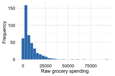
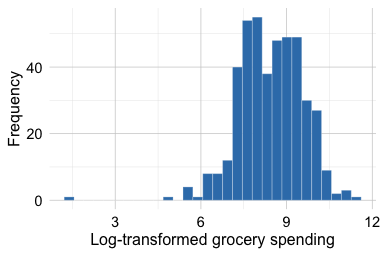
grocery spending variable before and after log transformation. The transformation compresses the long right tail and reduces the influence of very large values.
We apply the same transformation to all six spending variables:
customers_log = log1p(customers_subset)The log transformation reduces the influence of unusually large spending values, but it does not make K-means robust to extreme observations. Severe outliers may still affect Euclidean distances and centroid locations and should therefore be considered when interpreting the resulting clusters.
The transformed variables also differ in numerical range. Because K-means is distance-based, variables with larger ranges could contribute more strongly to the clustering simply because of their scale. As discussed in Section 3.6, scaling places the variables on a comparable basis before distances are calculated.
Here, we apply min-max scaling using the minmax() function from the liver package, which places each spending variable on the \([0,1]\) scale while preserving its ordering:
customers_mm = minmax(customers_log, col = "all")Other scaling approaches, such as z-score standardization, are also possible and may lead to somewhat different clustering solutions. This illustrates an important feature of clustering: transformation and scaling are not merely technical preliminaries. They determine how similarity is represented and can therefore influence the groups that emerge.
The transformed and scaled spending variables are now ready for K-means clustering. We next consider how many clusters provide a useful representation of the customer purchasing patterns.
Choosing the Number of Clusters
A key decision in clustering is choosing the number of clusters, \(k\). If too few clusters are used, important variation in customer purchasing behavior may be overlooked. If too many clusters are used, the resulting solution may become fragmented and difficult to interpret. Because clustering is an unsupervised method, this choice cannot be guided by predictive accuracy. Instead, we rely on internal criteria together with substantive interpretability.
We begin with the elbow method, which examines how the total within-cluster sum of squares (WCSS) changes as the number of clusters increases. As more clusters are added, WCSS decreases because observations are grouped into smaller and more homogeneous clusters. However, the improvement typically becomes smaller as \(k\) continues to increase. The aim is to identify a point beyond which adding more clusters yields only limited benefit.
To visualize this pattern, we use the fviz_nbclust() function from the factoextra package:
library(factoextra)

set.seed(42)
fviz_nbclust(customers_mm, kmeans, method = "wss", k.max = 10, nstart = 25) +
  geom_vline(xintercept = 3, linetype = 2, color = "gray")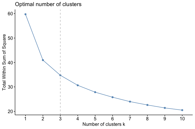
The elbow plot shows a sharp decrease in WCSS for small values of \(k\), followed by a more gradual decline. In this dataset, the curve begins to level off around \(k = 3\), suggesting that three clusters may provide a reasonable balance between simplicity and within-cluster cohesion.
The elbow method should be treated as a heuristic rather than as a definitive rule. Other internal criteria, such as silhouette scores or the gap statistic, can also provide useful information when comparing clustering solutions. In practice, however, the choice of \(k\) should also consider whether the resulting groups are coherent and meaningful in the context of the application. For this case study, the elbow plot suggests \(k = 3\) as a reasonable and relatively simple choice. We therefore proceed with three clusters and later examine whether the resulting customer segments are sufficiently distinct and substantively interpretable.
Practice: Compare K-means solutions for \(k = 2\), \(3\), \(4\), and \(5\). Which value provides the best balance between cohesion, separation, and interpretability?
Performing K-means Clustering
With the number of clusters selected, we now apply the K-means algorithm to segment the customers into three groups. We use the kmeans() function from base R, which implements the standard K-means procedure without requiring additional packages. The key arguments are the input data (x), the number of clusters (centers), and the number of random initializations (nstart). Because K-means can converge to different local minima depending on the initial placement of the centroids, using multiple random starts makes the fitted solution more stable and reduces the risk of settling on a poor partition.
To ensure reproducibility, we set a random seed. We then fit the model using the transformed and scaled spending variables:
The resulting object contains several components that summarize the clustering solution. The cluster component records the cluster assignment for each customer, centers gives the cluster centroids in the transformed feature space, size reports the number of customers assigned to each cluster, and tot.withinss gives the total within-cluster sum of squares. This quantity is directly related to the K-means objective function introduced earlier: smaller values indicate that observations lie, on average, closer to their assigned centroids. Its value should therefore be interpreted relative to competing clustering solutions rather than in isolation.
As an initial check, we inspect the cluster sizes and the total within-cluster sum of squares:
customers_kmeans$size
   [1] 139  82 219
customers_kmeans$tot.withinss
   [1] 34.76902
The cluster sizes show how the 440 customers are distributed across the three groups, while tot.withinss summarizes how tightly the observations are grouped around their respective centroids. Cluster size alone does not determine whether a clustering solution is good, but it provides a useful first check. Extremely small clusters may indicate outliers or an overly fragmented solution, whereas more balanced sizes may suggest broader and more interpretable customer segments. At the same time, a low within-cluster sum of squares should not automatically be taken as evidence of a meaningful clustering, since this quantity will generally decrease as more clusters are added. It must therefore be considered together with stability and interpretability.
Practice: Re-run K-means with a different random seed or a larger value of
nstart. How much do the cluster assignments, sizes, andtot.withinsschange?
Visualizing the Clusters
To obtain an initial visual impression of the clustering result, we use the fviz_cluster() function from the factoextra package:
fviz_cluster(customers_kmeans, customers_mm, geom = "point",
             ellipse.type = "norm", ggtheme = theme_minimal())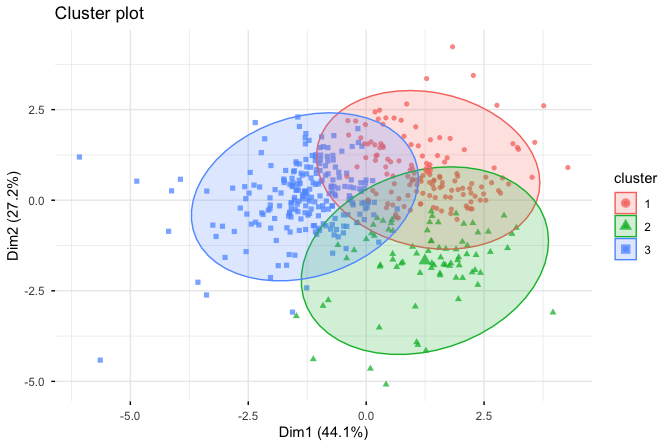
The resulting plot displays customers as points, with colors indicating cluster membership. The ellipses summarize the spread of the observations within each cluster. Because the dataset contains more than two variables, the figure is based on a projection of the data onto two principal components. This makes the clustering easier to inspect visually, but it is important to interpret the figure with caution: it is only a two-dimensional approximation of the structure in the full feature space. Visual separation in the projection does not prove strong separation in the original multidimensional data, just as apparent overlap in the plot does not necessarily imply poor clustering.
With this limitation in mind, the visualization is still useful as an exploratory aid. It helps us see whether the fitted clusters appear broadly distinct and whether some regions of the data show greater overlap than others. In this case, the plot suggests that the customer groups are reasonably differentiated, while also reminding us that the final assessment of the clustering should not rest on the projection alone. To understand what these groups mean substantively, we must examine their cluster profiles more closely. We turn to that interpretation next.
Interpreting the Clusters
After fitting the K-means model, the next step is to interpret what the clusters represent in substantive terms. Cluster labels such as 1, 2, and 3 are only numerical identifiers. On their own, they do not carry business meaning. To interpret the clusters, we attach the cluster labels to the original dataset, compare the average spending profiles across clusters, and then examine channel and region as external descriptive variables.
We begin by attaching the cluster assignments to the original data and inspecting the number of customers in each cluster:
customers_clustered = wholesale_customers
customers_clustered$cluster = factor(customers_kmeans$cluster)

table(customers_clustered$cluster)

     1   2   3
   139  82 219
The cluster sizes provide an initial summary of the solution. Extremely small clusters may indicate outliers or an overly fragmented solution, whereas broader clusters may suggest more general and interpretable customer groups.
Next, we compare the average annual spending in each product category within each cluster:
cluster_profiles = aggregate(. ~ cluster,
     data = customers_clustered[, c("cluster", selected_variables)], mean)

cluster_profiles
     cluster     fresh      milk   grocery    frozen detergents_paper delicassen
   1       1 16768.626 10863.453 13388.640 4200.6978        5181.3957  2821.1079
   2       2  3688.134  6985.683 12777.817  548.3537        5624.3171   882.8659
   3       3 12086.142  2134.753  2692.968 3300.4018         394.7443   942.5297
This summary is more interpretable than the transformed centroids returned by kmeans(), because it expresses the cluster profiles in the original spending units. The key question is comparative: which spending categories are relatively more prominent in each cluster?
Based on the cluster means, we can now interpret the groups more directly. Cluster 1 is characterized by comparatively high average spending on milk, grocery, and detergents_paper, while spending on fresh and frozen is less dominant relative to the other clusters. Cluster 2 shows stronger spending on fresh, frozen, and delicassen, suggesting a different purchasing profile. Cluster 3 appears more moderate or mixed, without the same degree of concentration in one particular subset of product categories. These descriptions are more informative than the numerical labels alone because they connect the clustering result back to substantive differences in purchasing behavior.
To support this interpretation further, we examine how customer type and region are distributed across the clusters:
table(Cluster = customers_clustered$cluster,
      Channel = customers_clustered$channel)
          Channel
   Cluster Horeca Retail
         1     52     87
         2     30     52
         3    216      3

table(Cluster = customers_clustered$cluster,
      Region = customers_clustered$region)
          Region
   Cluster Lisbon Oporto Other
         1     25     11   103
         2     12      9    61
         3     40     27   152
These tables do not define the clusters, since channel and region were not used to construct them. Instead, they provide external context that can help us understand whether the data-driven groups align with known business characteristics. For example, if the cluster with high spending on grocery-related categories is concentrated in one channel, that strengthens the interpretation of the group without making it circular.
Taken together, these summaries allow us to assign cautious descriptive labels to the clusters. In this case, labels such as grocery-oriented, fresh-food-oriented, and mixed spending are more appropriate than labels that sound fixed or definitive. Clustering does not reveal true customer types hidden inside the data. Rather, it provides an exploratory summary of purchasing behavior that may support interpretation and business decision-making.
To inspect the customers belonging to a specific cluster, we can subset the dataset using the cluster labels. For example, the following command lists the customers assigned to Cluster 1:
customers_clustered[customers_clustered$cluster == 1, ]This interpretation step is essential. The value of clustering lies not only in producing a partition of the data, but in determining whether the resulting clusters are coherent, interpretable, and useful for the problem at hand.
Practice: Assign a short descriptive label to each cluster. Which spending variables distinguish the clusters most clearly, and how do
channelandregionsupport your interpretation?
12.6 Chapter Summary and Takeaways
This chapter introduced clustering as a core method in unsupervised learning, used when no response variable is available and the goal is to identify structure in the data. Rather than predicting known outcomes, clustering groups observations according to similarity and provides an exploratory summary of multivariate patterns. Clustering should therefore be viewed as a tool for discovering potentially useful structure rather than as a method for recovering fixed or guaranteed groups.
The chapter focused on K-means clustering, which partitions observations by assigning them to the nearest centroid and iteratively updating those centroids to reduce the within-cluster sum of squares. The resulting solution depends on several analytical choices, including the representation of the data, the number of clusters, and the initialization of the algorithm. For distance-based methods such as K-means, feature selection, transformation, and scaling directly affect the geometry of the data and therefore the clusters that emerge. Likewise, the choice of \(k\) is heuristic and context-dependent, so internal criteria such as the elbow method and silhouette scores should be considered together with stability and substantive interpretability.
The wholesale_customers case study illustrated these ideas by segmenting customers according to purchasing behavior. After preparing the spending variables, we selected a reasonable value of \(k\), fitted a K-means model, and interpreted the resulting segments using their spending profiles together with channel and region as external descriptive variables. The chapter also briefly introduced hierarchical clustering, density-based clustering, and mixture models, emphasizing that different clustering methods reflect different assumptions about what constitutes a cluster.
Although clustering differs from the supervised methods developed earlier in the book, it still fits within the broader Data Science Workflow. Data Understanding and Exploration and Data Preparation for Modeling are especially important because they determine how similarity is represented, while Modeling constructs the clusters and Model Evaluation relies on cohesion, separation, stability, and substantive interpretation rather than predictive accuracy. Overall, clustering is exploratory rather than confirmatory, and its value lies not in producing a partition by itself, but in obtaining groups that are sufficiently stable, interpretable, and meaningful to support the analytical objective.
12.7 Exercises
These exercises reinforce the main ideas of the chapter, with emphasis on data preparation, the choice of \(k\), assessment of clustering solutions, and interpretation. The exercises use the red_wines dataset from the liver package unless stated otherwise.
Conceptual Questions
What is clustering, and how does it differ from classification?
Why is clustering considered an unsupervised learning method?
Explain the idea of high within-cluster similarity and high between-cluster separation. Why are both desirable in a clustering solution?
What role does a similarity or distance measure play in clustering?
Why is Euclidean distance commonly used in K-means clustering?
Describe the role of centroids in K-means clustering.
What objective function does K-means attempt to minimize?
Why can different random initializations lead to different K-means solutions?
What is meant by saying that K-means may converge to a local minimum?
Why can data preparation choices such as transformation and scaling change the clustering result?
Why is K-means especially sensitive to variables measured on different scales?
Why may K-means perform poorly when clusters are elongated, overlapping, or very unequal in size?
What is the elbow method, and why should it be treated as a heuristic rather than as a definitive rule?
How does the silhouette score help assess a clustering solution?
Why should cluster interpretation be treated cautiously rather than as the discovery of true categories hidden in the data?
Briefly describe one situation in which hierarchical clustering, density-based clustering, or mixture models may be more appropriate than K-means.
Hands-On Practice: K-means with the red_wines Dataset
The red_wines dataset contains chemical measurements for red wines together with a quality score. Use the chemical variables for clustering and reserve quality as an external descriptive variable for interpretation.
- Load the
red_winesdataset from the liver package and inspect its structure.
Summarize the dataset using
summary(). Are any missing values present? What do the summaries suggest about differences in scale, skewness, or unusually large observations?Formulate the analytical objective for this clustering analysis. What characteristics would make the resulting wine clusters useful and interpretable?
Identify the chemical variables that will be used as clustering inputs and reserve
qualityfor interpretation after clustering. Create an object containing only the clustering variables.
Examine the distributions of the clustering variables. Which variables appear strongly skewed?
Choose one skewed variable and visualize its distribution before and after applying a suitable transformation. What changes do you observe?
Transform the clustering variables if needed, store the result as
red_wines_prepared, and briefly justify your choice.Scale the variables in
red_wines_preparedbefore applying K-means and store the resulting data asred_wines_scaled. Explain why scaling is important in this setting.Use the elbow method on the prepared and scaled clustering variables to examine plausible values of \(k\).
library(factoextra)
fviz_nbclust(red_wines_scaled, kmeans, method = "wss", k.max = 10)
Compute the average silhouette score for \(k = 2, 3, 4,\) and \(5\) using
red_wines_scaled.Compare the elbow plot and silhouette results. Do they suggest the same value of \(k\), or do they point to different reasonable choices?
Based on the numerical evidence and your judgment about interpretability, choose a value of \(k\) for the remaining exercises. Justify your choice briefly.
Fit a K-means model to
red_wines_scaledusing your chosen value of \(k\). Use a fixed random seed and a sufficiently large value ofnstart.Report the cluster sizes. Do any clusters appear unusually small or disproportionately large?
Report the total within-cluster sum of squares (
tot.withinss). What does this quantity measure in the context of K-means?Refit the model with a different random seed or a larger value of
nstart. Do the cluster sizes, assignments, ortot.withinsschange noticeably? What does this suggest about the stability of the solution?Visualize the fitted clusters. If you use a two-dimensional projection, explain why the figure should be interpreted cautiously.
Attach the cluster labels to the original
red_winesdataset and compute the mean chemical profile of each cluster.Compare the cluster profiles and describe how the clusters differ from one another. Which chemical variables appear most useful for distinguishing the groups?
Compare the distribution of
qualityacross clusters. Do some clusters tend to contain higher-quality wines, and why should this be interpreted cautiously?Assign descriptive labels to the clusters based on their chemical profiles. Why should these labels remain tentative?
Compare clustering solutions under two different data preparation choices, such as unscaled versus scaled data. How do the resulting clusters differ?
Compare your solution with nearby values of \(k\). Does your original choice still seem reasonable in terms of cohesion, separation, stability, and interpretability?
Extensions and Reflection
Apply another clustering method, such as hierarchical clustering, to the same chemical variables. How does the result compare with K-means?
Reflect on the
red_winesanalysis. Which decisions most influenced the clustering, and what additional information would you want before using the results in practice?