| Outcome Type | Response Distribution | Link Function | Model |
|---|---|---|---|
| Continuous outcome | Normal | Identity | Linear regression |
| Binary outcome | Bernoulli/binomial | Logit | Logistic regression |
| Count outcome | Poisson | Log | Poisson regression |
9 Generalized Linear Models
Mathematics is the art of giving the same name to different things.
Many data science problems ask not only how much we expect, but whether an event will occur or how many times it will occur. Will a loan application be approved? Will a patient have a disease? How many service calls will a customer make within a given period? These questions involve binary or count outcomes rather than continuous responses and motivate the use of generalized linear models.
Chapter 7 introduced the foundations of statistical inference, including estimation, uncertainty, confidence intervals, and hypothesis testing. In Chapter 8, we applied these ideas to regression models for continuous outcomes, relating a numerical response variable to a set of predictors, interpreting coefficient estimates, quantifying uncertainty, and generating predictions. We now extend this regression framework to settings in which the response is binary or represents a count.
Ordinary linear regression does not naturally accommodate these types of outcomes. For binary responses, it can produce fitted values below 0 or above 1, even though the conditional mean is a probability and must lie between 0 and 1. For count responses, it does not respect the discrete and non-negative structure of the data. In both cases, the variability of the response is also linked to its mean in ways that differ from the constant-variance setting of ordinary linear regression. Applying a linear regression model mechanically can therefore lead to predictions and interpretations that are difficult to justify.
Generalized linear models address these limitations while preserving the central idea of regression: relating an outcome to a set of predictors in an interpretable way. We first introduce the general structure of generalized linear models, then study logistic regression for binary outcomes and Poisson regression for count outcomes. We conclude with a case study on predicting online purchase intention, following the Data Science Workflow introduced in Chapter 1. Together, these sections show how the regression framework can be extended beyond continuous outcomes to support interpretation, prediction, and decision-making.
What This Chapter Covers
This chapter introduces generalized linear models as a framework that extends ordinary linear regression to response types such as binary and count outcomes. Building on the statistical inference concepts introduced in Chapter 7 and the regression framework developed in Chapter 8, we examine how regression models can be adapted when the structure of the response differs from that of a continuous outcome. We begin by explaining why ordinary linear regression is unsuitable for binary and count responses and then introduce the three components of a generalized linear model: the response distribution, the linear predictor, and the link function.
We then study two important members of the GLM family. Logistic regression is used for binary outcomes and allows us to model event probabilities, interpret coefficients through odds ratios, and convert predicted probabilities into class predictions when a decision threshold is required. Poisson regression is used for count outcomes and allows us to model expected counts, interpret multiplicative predictor effects, and consider practical issues such as overdispersion.
Finally, we apply logistic regression in a case study on predicting online purchase intention. The case study emphasizes probability-based prediction and compares classification models using ROC curves and the area under the curve, introduced in Chapter 5. By the end of the chapter, you will be able to recognize when generalized linear models are appropriate, fit and interpret logistic and Poisson regression models in R, and evaluate probability-based classifiers within an applied data science workflow.
9.1 From Linear Regression to Generalized Linear Models
Ordinary linear regression provides the starting point for much of regression modeling, but its assumptions are most appropriate for continuous responses. To extend regression to binary and count outcomes, we need models that match the structure of the response and relate predictors to the expected outcome on an appropriate scale. This section introduces that extension by first explaining why ordinary linear regression is not enough for these settings and then presenting the three components of a generalized linear model.
Why Linear Regression Is Not Enough
Linear regression is a powerful starting point because it gives us a clear way to relate a response variable to a set of predictors. However, its assumptions are closely tied to continuous outcomes. When the response is binary or count-based, a standard linear regression model may no longer respect the basic structure of the outcome.
For a binary response, the quantity of interest is usually a probability. A model for such an outcome should therefore produce fitted values between 0 and 1. Linear regression does not guarantee this. It can return fitted values below 0 or above 1, which cannot be interpreted as probabilities. In addition, the variability of a binary response depends on the probability of the event. If the event probability is \(p\), then the variance is \(p(1-p)\), so the variability is smaller when \(p\) is close to 0 or 1 and larger when \(p\) is close to 0.5. This differs from the constant-variance assumption used in ordinary linear regression.
For count data, the response records how many times an event occurs. Counts are non-negative integers, so a model for their expected value should not produce negative fitted values. Linear regression does not impose this restriction. Count outcomes also often become more variable as their expected value increases. For example, the number of service calls made by customers is likely to vary more among customers with high expected usage than among customers with very low expected usage.
These limitations suggest that regression models should be adapted to the type of response variable being analyzed. For binary outcomes, we need a model for event probabilities. For count outcomes, we need a model for non-negative expected counts. Generalized linear models provide a unified framework for making these adaptations while preserving the central regression idea of relating an outcome to a set of predictors.
Rather than treating binary and count outcomes as cases outside regression, generalized linear models extend regression by combining a suitable response distribution, a linear predictor, and a link function. The next subsection introduces these three components more formally.
The Three Components of a Generalized Linear Model
A generalized linear model, often abbreviated as GLM, is defined by three connected components. Together, these components specify how the response is distributed, how the predictors enter the model, and how the expected response is linked to those predictors.
The first component is the random component. This specifies the probability distribution of the response, conditional on the predictors. In ordinary linear regression, the response is continuous and is typically modeled using a normal distribution around its conditional mean. In a generalized linear model, by contrast, we choose a distribution that matches the type of outcome being analyzed. For individual binary responses, the Bernoulli distribution is the relevant special case of the binomial distribution. For count data, the Poisson distribution is often used as a starting point.
The second component is the systematic component. This is the linear predictor, \[ \eta = \beta_0 + \beta_1 x_1 + \cdots + \beta_p x_p. \] Here, \(\beta_0, \beta_1, \dots, \beta_p\) are coefficients and \(x_1, x_2, \dots, x_p\) are predictors. This part of the model closely resembles the regression equations introduced in Chapter 8. It preserves the central regression idea that predictors combine linearly, although not necessarily on the original scale of the response.
The third component is the link function. This function connects the conditional mean of the response to the linear predictor. If we let \(\mu = \mathbb{E}(Y \mid x_1, \dots, x_p)\) denote the expected response for a given set of predictor values, then a generalized linear model has the form \[ g(\mu) = \eta. \] Here, \(g(\cdot)\) is the link function. Its role is to transform the mean response to a scale on which a linear relationship with the predictors is appropriate.
In ordinary linear regression, the link function is the identity link, so that \[ \mu = \eta. \] This means that the expected response is modeled directly as a linear function of the predictors. In logistic regression, the link function is the logit, which maps a probability to the log-odds scale. In Poisson regression, the link function is the logarithm, which maps a positive expected count to the real line.
Taken together, these three components show that generalized linear models do not replace regression, but extend it. Ordinary linear regression can itself be viewed as a special case of the GLM framework, with a normal response distribution and the identity link. Logistic and Poisson regression follow the same general structure while adapting it to binary and count outcomes.
Common GLMs for Different Outcome Types
The three GLM components come together differently depending on the type of response variable being modeled. In practice, this means choosing a response distribution that matches the outcome and a link function that connects the conditional mean of the response to the linear predictor. Table Table 9.1 summarizes the main cases considered in this chapter.
For a continuous response, the normal distribution together with the identity link gives the ordinary linear regression model developed in Chapter 8. For a binary response, the Bernoulli distribution for individual outcomes, or more generally the binomial distribution, combined with the logit link gives logistic regression. For a count response, the Poisson distribution combined with the log link gives Poisson regression.
This comparison highlights an important point: logistic and Poisson regression are not isolated methods unrelated to linear regression. They belong to the same general framework. What changes across these models is the response distribution and the link function used to connect the conditional mean of the response to the predictors. In this way, generalized linear models provide a unified language for regression across different types of outcomes.
This framework guides the rest of the chapter. We begin with logistic regression, which applies these ideas to binary outcomes and shows how regression can be used to model event probabilities in a principled and interpretable way.
9.2 Logistic Regression for Binary Outcomes
Many important data science questions involve a binary outcome. Will a loan application be accepted? Will a patient respond to treatment? Will a transaction be classified as fraudulent? In each case, the response takes one of two possible values. Earlier in the book, we approached such problems from a classification perspective through methods such as k-Nearest Neighbors in Chapter 4 and the Naive Bayes classifier in Chapter 6. We now turn to a complementary model-based approach that places binary outcomes within the regression framework: logistic regression.
Logistic regression is one of the most widely used generalized linear models. Rather than modeling the binary response directly as a numerical value, it models the probability of an event. The model does this through a transformation that keeps fitted probabilities between 0 and 1, avoiding key problems of ordinary linear regression for binary data such as fitted values outside \([0,1]\) and an inappropriate linear relationship on the probability scale.
Let \(Y = 1\) denote the event of interest and let \(p = P(Y = 1)\) denote the probability that this event occurs. In a loan application setting, for example, the event of interest might be that a loan application is approved. In a medical setting, it might be that a patient responds to treatment. The specific event changes from one application to another, but the modeling idea remains the same: logistic regression models the probability of the event of interest.
Instead of modeling \(p\) directly as a linear function of the predictors, logistic regression first considers the odds of the event, \[ \text{odds} = \frac{p}{1-p}. \] The odds compare the probability that the event occurs with the probability that it does not occur. If \(p = 0.8\), then the odds are \(0.8/0.2 = 4\), meaning that the event is four times as likely to occur as not to occur.
Because odds are always positive, we take their natural logarithm to obtain the log-odds, also called the logit: \[ \text{logit}(p) = \log\left(\frac{p}{1-p}\right). \] This transformation maps probabilities in the interval \((0,1)\) to the entire real line. Logistic regression then models the transformed probability as a linear function of the predictors: \[ \text{logit}(p) = \beta_0 + \beta_1 x_1 + \cdots + \beta_p x_p. \]
This is the logistic regression model. It states that the predictors have a linear effect on the log-odds scale. Although the model is linear in the coefficients, the relationship between the predictors and the probability itself is nonlinear. Solving the equation above for \(p\) gives the inverse-logit form: \[ p = \frac{ e^{\beta_0 + \beta_1 x_1 + \cdots + \beta_p x_p} }{ 1 + e^{\beta_0 + \beta_1 x_1 + \cdots + \beta_p x_p} }. \] This expression guarantees that predicted probabilities always lie between 0 and 1. That is the key reason logistic regression is appropriate for binary outcomes. It preserves the central regression idea of relating an outcome to predictors, but does so on a scale that matches the structure of binary data. In this way, logistic regression provides a statistically coherent and interpretable framework for modeling event probabilities.
Fitting and Interpreting a Logistic Regression Model in R
We now fit a logistic regression model in R using the loan dataset from the liver package. This dataset was introduced earlier in Chapter 6, where we used it to illustrate the Naive Bayes classifier. Here, we return to the same binary prediction problem from a regression perspective. Our goal is to model the loan outcome loan_status using applicant characteristics and financial indicators.
We begin by loading the dataset:
The dataset contains 4269 observations and 13 variables. The response variable is loan_status, while the remaining variables describe aspects of the applicant’s financial profile, asset values, and background.
Before fitting the model, it is useful to inspect the levels of the response variable. In logistic regression with a two-level factor response, R treats the second factor level as the modeled event by default. We therefore define the event of interest explicitly. Since we want to model the probability that a loan is approved, we set "rejected" as the reference category:
levels(loan$loan_status)
   [1] "approved" "rejected"

loan$loan_status = relevel(loan$loan_status, ref = "rejected")

levels(loan$loan_status)
   [1] "rejected" "approved"
Because "rejected" is the reference level, the model estimates the probability that loan_status = "approved". All coefficient interpretations in this example therefore refer to the odds of loan approval.
To keep the example concise, we include all available predictors except loan_id, which serves only as an identifier and does not carry predictive meaning. This allows us to focus on model fitting and interpretation without listing each predictor individually. We first define the model formula:
formula_loan = loan_status ~ . - loan_idWe then fit the logistic regression model using the glm() function. The argument family = binomial tells R to fit a generalized linear model for a binary response using the logit link:
glm_loan = glm(formula = formula_loan, data = loan, family = binomial)To inspect the fitted model, we use:
summary(glm_loan)

   Call:
   glm(formula = formula_loan, family = binomial, data = loan)

   Coefficients:
                              Estimate Std. Error z value Pr(>|z|)
   (Intercept)              -1.131e+01  4.377e-01 -25.833  < 2e-16 ***
   no_of_dependents         -1.780e-02  3.487e-02  -0.510   0.6097
   educationnot-graduate    -1.153e-01  1.183e-01  -0.975   0.3298
   self_employedyes          6.739e-02  1.181e-01   0.570   0.5684
   income_annum             -6.137e-07  9.081e-08  -6.758  1.4e-11 ***
   loan_amount               1.447e-07  1.812e-08   7.986  1.4e-15 ***
   loan_term                -1.516e-01  1.144e-02 -13.253  < 2e-16 ***
   cibil_score               2.483e-02  8.385e-04  29.612  < 2e-16 ***
   residential_assets_value  2.923e-09  1.187e-08   0.246   0.8055
   commercial_assets_value   1.903e-08  1.729e-08   1.101   0.2711
   luxury_assets_value       3.130e-08  1.749e-08   1.789   0.0735 .
   bank_asset_value          5.076e-08  3.342e-08   1.519   0.1287
   ---
   Signif. codes:  0 '***' 0.001 '**' 0.01 '*' 0.05 '.' 0.1 ' ' 1

   (Dispersion parameter for binomial family taken to be 1)

       Null deviance: 5660.7  on 4268  degrees of freedom
   Residual deviance: 1877.7  on 4257  degrees of freedom
   AIC: 1901.7

   Number of Fisher Scoring iterations: 7
The output reports the estimated coefficients, their standard errors, the corresponding z-statistics, and p-values. Each estimated coefficient \(b_j\) describes the direction and magnitude of the relationship on the log-odds scale, while its standard error reflects the uncertainty associated with that estimate. The z-statistic and p-value provide evidence for assessing whether the corresponding population coefficient \(\beta_j\) differs from zero. As discussed in Chapters 7 and 8, confidence intervals provide another way to quantify uncertainty; in logistic regression, exponentiating their endpoints gives confidence intervals for the corresponding odds ratios.
Each estimated coefficient in a fitted logistic regression model can be interpreted on two closely related scales. On the model scale, the estimated coefficient \(b_j\) describes the change in the log-odds of loan approval associated with a one-unit increase in predictor \(x_j\), holding the other predictors fixed. After exponentiation, the coefficient can be interpreted as an odds ratio. For a numeric predictor \(x_j\), exponentiating the estimated coefficient \(b_j\) gives \(e^{b_j}\), which represents the estimated multiplicative change in the odds of loan approval associated with a one-unit increase in \(x_j\), holding the other predictors fixed.
For example, according to the fitted model, the coefficient of loan_term is -0.152. The corresponding odds ratio is \(e^{-0.152}\) = 0.859. This means that a one-unit increase in loan_term multiplies the odds of loan approval by about 0.859, holding all other predictors fixed. If the odds ratio is greater than 1, the predictor increases the odds of approval; if it is less than 1, the predictor decreases the odds of approval.
For categorical predictors such as education or self_employed, the interpretation is relative to the reference category. In that case, the exponentiated coefficient compares the odds of loan approval in one category with the odds of loan approval in the reference category, holding the other predictors fixed. More generally, when factor variables are included in a model formula, R automatically creates the required indicator variables and uses one level as the reference category.
At this stage, we fit the model using the full dataset because our main goal is to understand model specification and coefficient interpretation. Later in this chapter, we return to logistic regression in a predictive setting and evaluate its out-of-sample performance in a fuller case study on predicting online purchase intention.
Taken together, these results show how logistic regression combines model estimation with interpretable coefficient analysis, allowing us to examine how individual predictors relate to the odds of loan approval.
Practice: Apply stepwise regression, as introduced in Section 8.5, to the logistic regression model. Compare the selected model with the full model in terms of retained predictors and interpretability. What does the reduced model suggest about the main factors related to loan approval?
From Estimated Probabilities to Classification Decisions
A logistic regression model produces predicted probabilities rather than class labels directly. These probabilities describe the estimated chance that each observation belongs to the modeled event category. In many applications, this probabilistic output is already useful, since it allows us to rank observations by estimated risk or likelihood.
Predicted probabilities can be obtained using predict() with type = "response":
round(predict(glm_loan, newdata = loan[1:5, ], type = "response"), 3)
       1     2     3     4     5
   0.998 0.078 0.211 0.420 0.002
These values represent the model’s estimated probabilities for the event corresponding to the second level of loan_status, which here is approved. Since we set "rejected" as the reference category in the previous subsection, the modeled event is loan approval. In other words, these values give the estimated probability that each selected loan application will be approved. For example, for the first application in the loan dataset, the estimated probability of approval is 0.998.
In some situations, predicted probabilities are the final quantity of interest. In others, however, we need a class prediction such as approved or rejected. To move from probabilities to class labels, we choose a decision threshold. The most common choice is 0.5: if the predicted probability of approval is at least 0.5, we classify the application as approved; otherwise, we classify it as rejected.
loan_probs = predict(glm_loan, newdata = loan, type = "response")

loan_pred_05 = ifelse(loan_probs >= 0.5, "approved", "rejected")
loan_pred_05 = factor(loan_pred_05, levels = levels(loan$loan_status))

table(loan_pred_05)
   loan_pred_05
   rejected approved
       1611     2658
The threshold is applied to the probability of the modeled event. In this example, the modeled event is loan approval, so lowering the threshold makes it easier for an application to be classified as approved, while raising the threshold makes the classification rule more selective.
Although a threshold of 0.5 is common, it is not always the most appropriate choice. The preferred threshold depends on the goals of the application and the relative consequences of different types of errors. In loan approval, for example, a lender may choose a higher threshold for approval if the cost of approving a risky application is especially high. Conversely, a lower threshold may be preferred if the cost of rejecting applicants who would in fact repay the loan is considered greater. The threshold should therefore reflect the practical balance between caution and opportunity in the decision process. If the threshold is chosen by comparing predictive performance across candidate values, that choice should be made using training or validation data rather than the final test set.
This highlights one of the main strengths of logistic regression. It separates the task of estimating probabilities from the task of making decisions. The model provides estimated probabilities, and the analyst selects a threshold that reflects the practical context. In the case study later in this chapter, we evaluate probability-based classifiers using ROC curves and the area under the curve, which allow us to assess classification performance across all possible thresholds rather than relying on a single cutoff.
Logistic regression therefore serves two closely related purposes. It is a regression model for binary outcomes, and it is also a classification tool that yields interpretable probabilities. This combination of interpretability, flexibility, and practical usefulness explains why logistic regression remains one of the most important methods for binary data analysis.
Practice: Generate predicted probabilities for the
loandataset and classify applications using thresholds of 0.5 and 0.3. How does lowering the threshold affect the number of approvals and the trade-off between approving risky applicants and rejecting applicants who might repay the loan?
9.3 Poisson Regression for Count Outcomes
Not all response variables describe whether an event occurs. In many applications, the outcome records how many times something happens within a fixed period or setting. Examples include the number of doctor visits, the number of insurance claims, the number of purchases made in a week, or the number of website visits in an hour. In Section 8.9, for example, we modeled hourly bike rental demand using the variable bike_count, which records the number of bikes rented in each hour. Outcomes of this kind are not continuous and are not simply binary. They are counts, and they require a model that respects their discrete, non-negative nature.
Poisson regression is one of the most important generalized linear models for this setting. It extends the regression framework to responses that represent event frequencies, allowing us to relate expected counts to a set of predictors in a structured and interpretable way. Just as logistic regression adapts regression to binary outcomes, Poisson regression adapts it to count outcomes. Revisiting bike_count from Section 8.9 will therefore help us see how a generalized linear model can sometimes provide a more natural representation of a count response than ordinary linear regression.
An important consideration in count modeling is the amount of exposure associated with each observation. The basic Poisson regression model presented here is most directly applicable when observations represent comparable periods or opportunities for events to occur. When exposure differs, such as when individuals are observed for different lengths of time, these differences can be incorporated into the model, commonly through an offset. In the bike-demand example, each observation represents one hour, so the exposure period is comparable across observations.
This matters because ordinary linear regression is not well suited to count data. A linear model can produce fitted values that are negative, even though counts must be non-negative. It also assumes a constant variance, whereas count outcomes often become more variable as their expected value increases. In addition, count data are often right-skewed, with many small values and fewer large ones. These features make the normal-error framework of linear regression less appropriate.
Poisson regression addresses these limitations by modeling the expected count through a distribution and link function designed for count outcomes. It is based on the Poisson distribution, named after the French mathematician Siméon Denis Poisson (1781–1840), who studied models for the number of events occurring within a fixed interval. If \(Y\) follows a Poisson distribution with parameter \(\lambda > 0\), then its probability mass function is \[ P(Y = y) = \frac{e^{-\lambda}\lambda^y}{y!}, \qquad y = 0,1,2,\dots \] where \(\lambda\) is the expected count. A key feature of the Poisson distribution is that its mean and variance are both equal to \(\lambda\): \[ \mathbb{E}(Y) = \lambda, \qquad \text{Var}(Y) = \lambda. \]
To relate the expected count to predictors, Poisson regression uses the log link: \[ \log(\lambda) = \beta_0 + \beta_1 x_1 + \beta_2 x_2 + \dots + \beta_m x_m. \] Here, \(\beta_0, \beta_1, \dots, \beta_m\) denote the model coefficients, following the same notation used for population regression coefficients in Chapter 8. The model states that the logarithm of the expected count is a linear function of the predictors. Solving for \(\lambda\) gives \[ \lambda = e^{\beta_0 + \beta_1 x_1 + \beta_2 x_2 + \dots + \beta_m x_m}. \]
This formulation guarantees that the expected count is always positive. It also implies that predictors act multiplicatively on the original count scale, even though their effects are additive on the log scale. When the model is fitted to observed data, the unknown coefficients \(\beta_j\) are estimated by coefficients denoted by \(b_j\), consistent with the notation used in Chapter 8. In this way, Poisson regression provides a statistically coherent and interpretable framework for modeling count outcomes.
Fitting and Interpreting a Poisson Regression Model for Bike Demand
In Section 8.9, we modeled hourly bike rental demand using linear regression, including nonlinear terms and a square-root transformation of the response. That analysis showed that linear regression can provide a useful approximation for this problem. At the same time, the response variable bike_count records the number of bike rentals in each hour, so it is fundamentally a count outcome. This makes Poisson regression a natural alternative to consider.
To make the comparison with Section 8.9 meaningful, we reproduce the same chronological training-test split used there. Before creating the split, we perform only fixed operations that do not depend on patterns observed in the response: we parse date, retain functioning days, order the observations chronologically by date and hour, and derive weekday from the calendar date. We then assign the first 80% of the observations to the training set and reserve the remaining 20% as the test set.
The model-development choices made in Chapter 8 were based on the training data. These included treating hour as a categorical predictor, using a quadratic term for temperature, and applying a square-root transformation to bike_count for the linear regression model. We reuse those established choices here so that the linear and Poisson models are compared under a consistent modeling setup. The Poisson model, however, is fitted directly to the original bike_count response because it models expected counts without requiring the square-root transformation.
We now fit a Poisson regression model using the same candidate predictor specification. Unlike the linear model, which models the square root of bike_count, the Poisson model uses the original count response:
The argument family = poisson tells R to use a Poisson response distribution together with the default log link. The expected number of bike rentals is therefore modeled directly as a positive quantity. As an exploratory model-simplification step, we also apply the stepwise procedure introduced in Chapter 8. Importantly, this procedure uses only the training data:
stepwise_reg_glm = step(full_reg_glm, direction = "both", trace = FALSE)The fitted model can be examined using summary(stepwise_reg_glm), which reports the estimated coefficients, their standard errors, the corresponding z-statistics, and p-values. Because the complete output is lengthy, we do not reproduce it here. Instead, we focus on the interpretation of the fitted coefficients.
For example, the estimated coefficient of temperature is 0.061. Because Poisson regression uses the log link, this coefficient describes the estimated change in the log of the expected bike count associated with a one-unit increase in temperature, holding the remaining predictors fixed. Exponentiating the coefficient gives 1.063, indicating that a one-unit increase in temperature multiplies the expected number of bike rentals by approximately this factor. Equivalently, this corresponds to an estimated change of about 6.3% in the expected count, holding the other predictors fixed.
For categorical predictors, interpretation is relative to a reference category. For example, the coefficient for holidayno compares non-holidays with the reference category holidayyes, holding the remaining predictors fixed. Exponentiating this coefficient gives the estimated multiplicative difference in expected bike rentals between non-holidays and holidays.
More generally, each estimated coefficient can be interpreted on two related scales. For a numerical predictor \(x_j\), the estimated coefficient \(b_j\) represents the change in the log of the expected count associated with a one-unit increase in \(x_j\), holding the other predictors fixed. Exponentiating the coefficient gives \(e^{b_j}\), which represents the estimated factor by which the expected count changes for a one-unit increase in \(x_j\).
After the model-development steps have been completed, we use the reserved test set for final predictive evaluation. Predicted expected counts from the stepwise Poisson model are obtained using predict() with type = "response":
pred_stepwise_glm = predict(stepwise_reg_glm, newdata = test_bike, type = "response")These values are the model’s estimated expected numbers of bike rentals for the test observations. Because Poisson regression predicts expected counts, the predicted values do not need to be integers. They represent expected demand rather than the realized number of rentals in a particular hour.
We can now compare the Poisson regression model with the linear regression model from Section 8.9 on the original bike_count scale. For the linear model, predictions are first obtained on the square-root scale and then transformed back to the original count scale. We summarize predictive performance using RMSE and predictive \(R^2\):
                      Model     RMSE        R2
   1  Stepwise linear model 333.8172 0.6897669
   2 Stepwise Poisson model 289.1020 0.7673125
In this setting, the stepwise Poisson model achieves a lower predictive RMSE and a higher predictive \(R^2\) than the stepwise linear model from Chapter 8. In particular, the predictive RMSE decreases from about 333.8 to about 289.1, while the predictive \(R^2\) increases from about 0.69 to about 0.77. These results suggest that modeling bike_count directly as a count outcome provides a more effective representation for this particular prediction problem.
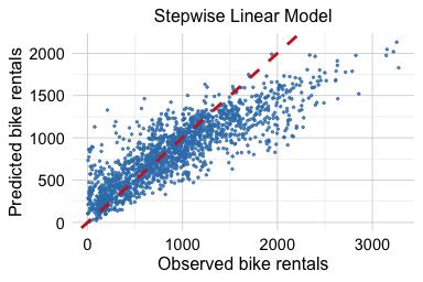
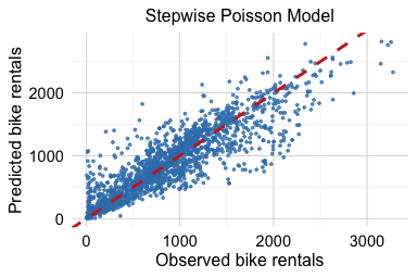
Figure 9.1 compares observed and predicted bike rentals for the stepwise linear model from Chapter 8.9 and the stepwise Poisson model. The Poisson model produces predictions that track the diagonal reference line more closely, which is consistent with its improved predictive performance on the test set. At the same time, Poisson regression should still be viewed as a starting point rather than a final answer for every count-data problem. Hourly demand data may exhibit overdispersion, meaning that the variability in the response exceeds what the Poisson model assumes. If substantial overdispersion is present, alternatives such as quasi-Poisson or negative binomial regression may be considered (Dobson and Barnett 2018). These extensions are beyond the main scope of this introductory chapter. It is therefore important to check model adequacy in practice, even when Poisson regression performs better than ordinary linear regression.
Practice: Revisit the
bike_demandanalysis in Section 8.9 and compare the stepwise linear and Poisson regression models. Interpret one numerical and one categorical predictor from the Poisson model on the log and expected-count scales. How does this interpretation differ from that of the linear regression model?
9.4 Case Study: Predicting Online Purchase Intention with Logistic Regression
Predicting whether an online browsing session will end in a purchase is a common classification problem in e-commerce. Accurate probability estimates can help businesses identify sessions with high conversion potential, target promotions more effectively, and better understand the factors related to customer purchasing behavior. In this case study, we ask a focused question: can an interpretable logistic regression model provide competitive probability-based predictions for online purchase intention?
The purchase_intention dataset comes from the UC Irvine Machine Learning Repository and is distributed with the liver package. It was described by Sakar et al. (2019) in the context of predicting online purchasing behavior. The response variable, revenue, records whether a session resulted in a completed transaction, while the predictors describe browsing behavior, session-level characteristics, and visitor-related features. This makes the dataset well suited for illustrating logistic regression in a realistic binary classification setting.
Following the Data Science Workflow introduced in Chapter 1 and illustrated in Figure 1.1, this case study proceeds from problem definition and data acquisition to data understanding and exploration, data preparation for modeling, modeling, and model evaluation. We first examine the purchase_intention data and establish the training-test split. Using the training data, we then fit a baseline logistic regression model, followed by a stepwise logistic regression model, and include the Naive Bayes classifier from Chapter 6 as a benchmark based on a different modeling principle. Once the models have been finalized, we compare their probability-based predictions on the reserved test set. The comparison considers predictive performance together with interpretability and parsimony.
Problem Definition
Online retailers routinely seek to understand which browsing sessions are most likely to end in a purchase. Identifying sessions with a high probability of conversion can help businesses target promotions more effectively, improve recommendation strategies, allocate marketing resources, and refine website design. This makes purchase intention a natural prediction problem in e-commerce: given information recorded during a browsing session, can we estimate whether that session will generate revenue?
From a modeling perspective, this is a binary classification problem. The outcome variable revenue records whether a session ended in a purchase (yes) or not (no). The predictors include behavioral variables, such as the number of pages visited and the time spent on different types of pages, together with session-level and visitor-level characteristics such as month, visitor_type, traffic_type, and weekend. Our aim is to estimate the probability of purchase for each session while also considering the trade-off between predictive performance and interpretability. For this reason, we begin with logistic regression, then consider a stepwise logistic regression model, and finally compare these models with Naive Bayes as an external benchmark.
Overview of the Dataset
The purchase_intention dataset is available through the liver package. We begin by loading the data and examining its structure, covering the Data Acquisition and Data Understanding and Exploration stages of the Data Science Workflow. Each observation corresponds to a single browsing session, and the modeling objective is to predict whether that session ended in a purchase (revenue = "yes" or "no"). The dataset combines behavioral measures with session-level and visitor-related characteristics, making it well suited for supervised classification in an e-commerce setting.
library(liver)

data(purchase_intention)

str(purchase_intention)
   'data.frame':    12330 obs. of  18 variables:
    $ administrative          : int  0 0 0 0 0 0 0 1 0 0 ...
    $ administrative_duration : num  0 0 0 0 0 0 0 0 0 0 ...
    $ informational           : int  0 0 0 0 0 0 0 0 0 0 ...
    $ informational_duration  : num  0 0 0 0 0 0 0 0 0 0 ...
    $ product_related         : int  1 2 1 2 10 19 1 0 2 3 ...
    $ product_related_duration: num  0 64 0 2.67 627.5 ...
    $ bounce_rates            : num  0.2 0 0.2 0.05 0.02 ...
    $ exit_rates              : num  0.2 0.1 0.2 0.14 0.05 ...
    $ page_values             : num  0 0 0 0 0 0 0 0 0 0 ...
    $ special_day             : num  0 0 0 0 0 0 0.4 0 0.8 0.4 ...
    $ month                   : Ord.factor w/ 10 levels "Feb"<"Mar"<"May"<..: 1 1 1 1 1 1 1 1 1 1 ...
    $ operating_systems       : Factor w/ 8 levels "1","2","3","4",..: 1 2 4 3 3 2 2 1 2 2 ...
    $ browser                 : Factor w/ 13 levels "1","2","3","4",..: 1 2 1 2 3 2 4 2 2 4 ...
    $ region                  : Factor w/ 9 levels "1","2","3","4",..: 1 1 9 2 1 1 3 1 2 1 ...
    $ traffic_type            : Factor w/ 20 levels "1","2","3","4",..: 1 2 3 4 4 3 3 5 3 2 ...
    $ visitor_type            : Factor w/ 3 levels "New_Visitor",..: 3 3 3 3 3 3 3 3 3 3 ...
    $ weekend                 : Factor w/ 2 levels "no","yes": 1 1 1 1 2 1 1 2 1 1 ...
    $ revenue                 : Factor w/ 2 levels "no","yes": 1 1 1 1 1 1 1 1 1 1 ...
The dataset consists of 12330 observations and 18 variables. The response variable, revenue, is binary and indicates whether the session resulted in a completed transaction. The predictors describe several aspects of the browsing session. Some variables summarize browsing behavior, including the number of administrative, informational, and product-related pages visited and the time spent on each type of page. Others capture session quality and commercial relevance, such as bounce_rates, exit_rates, page_values, and special_day. Additional variables describe session and visitor characteristics, including month, weekend, visitor_type, traffic_type, region, browser, and operating_systems.
Taken together, these predictors provide a rich description of online shopping sessions and the conditions under which purchases occur. For this case study, the dataset is already stored in an analysis-ready format, with categorical variables represented as factors and the binary outcome clearly defined. As a result, no additional cleaning is required before proceeding to Data Preparation for Modeling, where we establish the training-test split for model development and final evaluation.
Data Preparation for Modeling
To evaluate how well the models generalize to new data, we divide the purchase_intention dataset into separate training and test sets. The training set is used for model development, while the test set is reserved for final out-of-sample evaluation. This separation allows predictive performance to be assessed on observations that were not used when fitting or selecting the models.
Following the approach used elsewhere in the book, we use the partition() function from the liver package to create an 80% training set and a 20% test set. We also set a random seed to make the partition reproducible:
The split assigns most observations to the training set while leaving a substantial subset for model evaluation. Because revenue is the response variable, it is useful to check descriptively whether its class proportions are reasonably similar across the training and test sets:
prop.table(table(train_set$revenue))

          no       yes
   0.8437753 0.1562247
prop.table(table(test_set$revenue))

         no      yes
   0.851176 0.148824
The proportions indicate that the class distribution is similar across the two subsets. This descriptive check helps identify whether the random partition has produced an unusually different class balance in the test set. A formal hypothesis test is neither necessary nor appropriate for this purpose because the objective is to inspect the partition rather than test a population-level hypothesis.
No additional preprocessing is required for the models considered in this case study. The categorical predictors are already represented as factors, and the numerical predictors are ready for direct use. We therefore proceed to the Modeling stage using the training data, while keeping the test set reserved for final evaluation.
Practice: Repeat the partition using a 70% training set and a 30% test set. Compare the class proportions of
revenueacross the resulting subsets. How does changing the partitioning ratio affect the amount of data available for model development and final evaluation?
Fitting the Baseline Logistic Regression Model
We begin with logistic regression, which serves as the main modeling approach in this case study. Logistic regression is a natural choice because the response variable is binary and the goal is to estimate the probability that an online browsing session ends in a purchase.
We fit a baseline logistic regression model using all available predictors in the training set. In glm(), the argument family = binomial specifies a logistic regression model for a binary response using the logit link:
baseline_logit = glm(formula = revenue ~ ., data = train_set,family = binomial)The baseline model provides a reference specification that includes all available predictors. At this stage, our focus is on model development using the training data. We therefore do not yet generate predictions for the test set. Those predictions will be obtained only after all models have been finalized and will be used for final out-of-sample comparison in the Model Evaluation and Comparison subsection.
Practice: Inspect
summary(baseline_logit). Which predictors have positive or negative associations with the log-odds of purchase? Treat these patterns as in-sample model interpretation rather than out-of-sample performance.
Fitting the Stepwise Logistic Regression Model
The baseline logistic regression model includes all available predictors. While this provides a natural starting point, in practice we often ask whether a simpler model may provide a more parsimonious representation. A reduced model can be easier to interpret, easier to communicate, and more practical to use.
To investigate this possibility, we apply stepwise selection to the baseline logistic regression model using the training data. Stepwise selection compares a sequence of candidate models by adding or removing predictors and evaluating them using the Akaike Information Criterion (AIC). As discussed in Section 8.5, smaller AIC values indicate a better balance between model fit and model complexity. Here, we use bidirectional stepwise selection, which allows predictors to be both added and removed during the search.
stepwise_logit = step(baseline_logit, direction = "both", trace = 0)The resulting model is a reduced version of the baseline logistic regression model. Because stepwise selection is part of model development, it is performed entirely using the training data. We do not yet generate predictions for the test set. After all models have been finalized, the reserved test set will be used to compare their out-of-sample performance.
Stepwise selection should be interpreted cautiously. It is a data-driven search procedure, so the selected model can be sensitive to small changes in the data, and the usual coefficient summaries should not be interpreted as if the model had been specified in advance. In this case study, we use stepwise selection mainly as an exploratory tool for model simplification, not as a guarantee of better predictive performance or as a definitive procedure for identifying the true set of relevant predictors.
The final evaluation will show whether the reduced model retains similar discriminatory performance to the baseline logistic regression model. If it does, the more compact specification may offer a useful practical advantage through greater interpretability and parsimony.
Practice: Inspect the final stepwise model using
formula(stepwise_logit)orsummary(stepwise_logit). Which predictors were retained, and how does the model differ from the baseline logistic regression model? Why should the selected model be interpreted cautiously?
Fitting the Naive Bayes Model
To broaden the comparison beyond logistic regression, we also fit a Naive Bayes classifier. This model was introduced in Chapter 6 and provides a useful external benchmark because it is based on a different modeling principle. Whereas logistic regression models the probability of the outcome through the log-odds, Naive Bayes combines Bayes’ rule with a simplifying assumption about the predictors.
The defining assumption of Naive Bayes is that the predictors are conditionally independent given the class label. In practice, this assumption is often unrealistic, especially in a dataset such as purchase_intention, where behavioral variables such as page counts, browsing durations, and engagement measures are likely to be related. Even so, Naive Bayes often performs surprisingly well and is widely used as a simple and computationally efficient benchmark in classification problems.
We fit the model using the naive_bayes() function from the naivebayes package. As in the logistic regression models, we use revenue as the response variable and include all available predictors:
library(naivebayes)

bayes_fit = naive_bayes(formula = revenue ~ ., data = train_set, laplace = 1)
The argument laplace = 1 applies Laplace smoothing, which helps avoid zero estimated probabilities when some predictor values occur rarely within a class. At this stage, the Naive Bayes model is fitted using the training data only. We do not yet generate predictions for the test set. After all three models have been finalized, their probability-based predictions will be obtained on the reserved test set and compared using ROC curves and AUC in the Model Evaluation and Comparison subsection.
Naive Bayes is interpretable in a different sense from logistic regression: it summarizes how predictor distributions differ by class. However, it does not provide coefficient-based effect estimates or odds ratios. In this case study, its main role is to serve as a simple and computationally efficient benchmark based on assumptions that differ from those of logistic regression.
Practice: Many predictors in
purchase_intention, such as page counts and browsing durations, are likely to be correlated. Why does this create tension with the conditional independence assumption of Naive Bayes? Compare this with the assumptions made by logistic regression.
Model Evaluation and Comparison
We now evaluate the three finalized models on the reserved test set. At this stage, the model specifications and all model-development decisions have already been determined using the training data. The test set is used only for final out-of-sample assessment; we do not revise predictor sets, classification thresholds, or other modeling choices after examining test performance. This preserves the role of the test set described in Chapter 5.
We first store the true test-set labels and generate predicted probabilities from each of the three models:
For the two logistic regression models, type = "response" returns the estimated probability that revenue = "yes". For the Naive Bayes model, predict(..., type = "prob") returns probabilities for both outcome classes, so we select the "yes" column. These probability-based predictions allow the three models to be compared using the same evaluation framework.
The ROC curve plots the true positive rate against the false positive rate as the classification threshold varies. The AUC summarizes this curve into a single measure of discriminatory performance: values closer to 1 indicate stronger separation between the two outcome classes. Because purchase_intention is imbalanced, precision-recall curves can also provide a useful perspective on classifier performance. Here, however, we focus on ROC curves and AUC to compare discriminatory performance across thresholds for the three models.
We compute the ROC curves using the pROC package:
To compare the models visually, we plot all three ROC curves in a single figure:
ggroc(list(roc_logistic, roc_stepwise, roc_bayes), size = 0.8) +
  scale_color_manual(values = c("#377EB8", "#4DAF4A", "#E66101"),
    labels = c(paste("Logistic (AUC =", round(auc(roc_logistic), 3), ")"),
        paste("Stepwise (AUC =", round(auc(roc_stepwise), 3), ")"),
        paste("Naive Bayes (AUC =", round(auc(roc_bayes), 3), ")"))) +
  ggtitle("ROC Curves for Three Classification Models") +
  theme(legend.title = element_blank(), legend.position = c(.72, .3))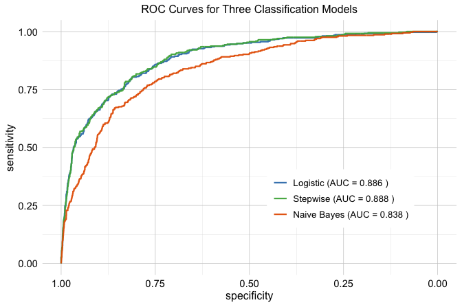
The ROC curves allow us to compare the models across a range of thresholds rather than at a single cutoff. In this case, the baseline logistic regression model and the stepwise logistic regression model achieve very similar AUC values, suggesting that the reduced model preserves most of the discriminatory information contained in the full model. This is a practically useful result, since a simpler model may offer nearly the same discriminatory performance while being easier to interpret and communicate.
Naive Bayes provides a useful external benchmark. Its performance shows whether a classifier based on a different modeling principle remains competitive on this dataset. Even with its simplifying conditional independence assumption, Naive Bayes can still provide a meaningful benchmark for comparison.
Taken together, the results illustrate a common applied trade-off. The baseline logistic regression model provides an interpretable reference point, the stepwise model examines whether a more parsimonious specification is sufficient, and Naive Bayes offers a contrasting benchmark. Comparing all three helps us evaluate not only discriminatory performance, but also interpretability, parsimony, and practical usefulness.
Practice: Compare the AUC values of the three models and interpret the differences. If two models achieve very similar AUC values, what considerations other than predictive performance might guide the choice between them?
9.5 Chapter Summary and Takeaways
In this chapter, we extended the regression framework beyond continuous outcomes by introducing generalized linear models. The central idea is to match the model to the structure of the response variable. A GLM combines a response distribution, a linear predictor, and a link function, allowing regression methods to be adapted to outcomes such as binary responses and counts.
For binary outcomes, we studied logistic regression. This model uses the logit link to relate predictors to the log-odds of an event while ensuring that predicted probabilities remain between 0 and 1. Logistic regression is therefore useful both as an interpretable regression model and as a classification tool. Its coefficients can be interpreted through odds ratios, and its predicted probabilities can be converted into class predictions when a decision threshold is required.
For count outcomes, we studied Poisson regression. This model uses the log link to relate predictors to the expected count and allows predictor effects to be interpreted multiplicatively on the original count scale. Poisson regression also relies on assumptions that should be assessed in practice, particularly the relationship between the mean and variance. Substantial overdispersion may indicate that alternatives such as quasi-Poisson or negative binomial regression should be considered.
The case study on online purchase intention illustrated how logistic regression can be used in a predictive setting. By comparing the baseline logistic regression model, the stepwise logistic regression model, and Naive Bayes using ROC curves and AUC, we emphasized that model choice should not depend on predictive performance alone. Interpretability, parsimony, and the decision context also influence the choice of a useful model. This reinforces a broader message of the Data Science Workflow: effective modeling requires matching the method not only to the structure of the data, but also to the purpose of the analysis.
Chapter 10 moves from generalized linear models to decision trees and random forests. Unlike the regression-based models developed in Chapters 8 and 9, tree-based methods can capture nonlinear relationships and interactions through recursive partitioning.
9.6 Exercises
These exercises reinforce the main ideas of the chapter through conceptual questions and practical applications in R. They focus on logistic regression, Poisson regression, and model comparison using datasets from the liver package.
Conceptual Understanding
Explain why ordinary linear regression is not appropriate for a binary response variable.
Explain why ordinary linear regression is not appropriate for count data.
What are the three main components of a generalized linear model?
What is the role of a link function in a generalized linear model?
Why does logistic regression use the logit link rather than the identity link?
Why does Poisson regression use the log link rather than the identity link?
What is an odds ratio, and how is it interpreted in logistic regression?
In Poisson regression, what does \(e^{\beta_j}\) represent for a predictor \(x_j\)?
What is overdispersion in the context of Poisson regression, and why can it be problematic?
Logistic regression and Poisson regression are both generalized linear models. What do they have in common, and how do they differ?
Hands-On Practice: Logistic Regression with the loan Dataset
data(loan, package = "liver")Inspect the structure of the
loandataset. Which variable is the response, and which variables are plausible predictors?Define loan approval as the modeled event by setting
"rejected"as the reference category ofloan_status. Fit a logistic regression model usingincome_annum,loan_amount, andcibil_score.Inspect the fitted model using
summary(). Interpret the estimated coefficient forcibil_scorein terms of the log-odds of loan approval.Exponentiate the estimated coefficients. Interpret the odds ratio for
cibil_scorein the context of loan approval.Extend the model by adding
educationandself_employed. How do the coefficient estimates and their statistical significance change?Use the extended model to estimate the probability of approval for an applicant with
income_annum = 5000000,loan_amount = 12000000,cibil_score = 750,education = "Graduate", andself_employed = "No".Use
partition()to create an 80% training set and a 20% test set. Fit the extended logistic regression model using the training data only.Apply stepwise selection using the training data. Which predictors are retained, and how does the selected model differ from the full model? Why should the selected model be interpreted cautiously?
Generate test-set probabilities from the full model and classify observations using thresholds of 0.5 and 0.3. Compare the resulting confusion matrices. How does lowering the threshold affect the classification errors?
Using a threshold of 0.5, compute accuracy, precision, recall, and F1-score on the test set for the full and stepwise models. Compare their out-of-sample performance, interpretability, and parsimony.
Hands-On Practice: Poisson Regression with the doctor_visits Dataset
data(doctor_visits, package = "liver")Inspect the structure of the
doctor_visitsdataset. Which variable is the response, and why is it suitable for Poisson regression?Fit a Poisson regression model predicting
visitsusingage,income,illness,reduced, andhealth.Inspect the fitted model using
summary(). Choose one numerical predictor and interpret its estimated coefficient on the log scale.Exponentiate the estimated coefficients. Choose two predictors and interpret their effects on the expected number of doctor visits.
Add a quadratic term for
ageusingageandI(age^2). Does the fitted model suggest a nonlinear relationship with the expected number of visits?Obtain fitted expected counts for three observations and compare them with the observed values. What does this suggest about the in-sample model fit?
Compare the first ten observed values of
visitswith their fitted values. How closely does the model represent these observations?Compute
deviance(model) / df.residual(model). Does the result suggest possible overdispersion?If substantial overdispersion is present, explain why quasi-Poisson or negative binomial regression might be considered instead.
Hands-On Practice: Model Comparison with purchase_intention
data(purchase_intention, package = "liver")Reproduce the 80%–20% training-test split used in the case study. Compare the class proportions of
revenuein the two subsets.Using the training set, fit a baseline logistic regression model predicting
revenuewith all available predictors. Inspect the fitted model.Apply stepwise selection to the baseline logistic regression model. Which predictors are retained, and how does the selected model differ from the full model?
Using the same training set, fit a Naive Bayes classifier with
revenueas the response and all available predictors.Generate test-set probabilities from the baseline logistic, stepwise logistic, and Naive Bayes models. Compare their ROC curves and AUC values. Which model performs best, and are the differences practically meaningful?
Reflection and Extension
- Describe a real-world problem with a binary or count outcome. Identify the response and plausible predictors, choose logistic or Poisson regression as a starting point, and explain which assumptions you would check.